This note illustrates a geometric interpretation of multivariate linear regression, which I have found to be the most intuitive way to think of regression problems. Given a feature matrix \(X\), and output vector \(y\), the objective of linear regression is to calculate a set of coefficients B that when linearly combined with \(X\) produces a new vector \(\hat{y}\). \( \hat{y} = X B \) Think of \(X\) as a m x n matrix, and \(y\) as a n-dimensional column vector. \( \hat{y} = \begin{bmatrix} a_{1,1} & a_{1,2} & \cdots & a_{1,n} \\ a_{2,1} & a_{2,2} & \cdots & a_{2,n} \\ \vdots & \vdots & \ddots & \vdots \\ a_{m,1} & a_{m,2} & \cdots & a_{m,n} \end{bmatrix}\\ \cdot \begin{bmatrix} a_{1,1} \\ a_{2,1} \\ .. 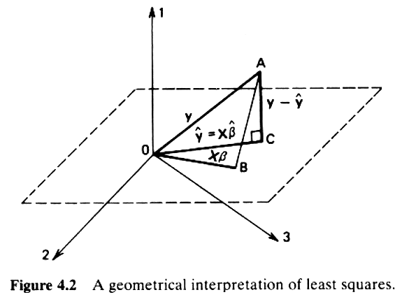\\ a_{m,1} \end{bmatrix}\) Geometrically, one can think of the output vector \(y\) as belonging to a m-dimensional ambient space. Since m is greater then the rank of \(X\), the feature matrix \(X\) contains n column vectors belonging to some hyperplane in m-dimensional space. The picture below illustrates a concrete example of this, with a m = 3 and n = 2. The \(y\) vector sits in 3-dimensional ambient space, and \(X\) consists of two 3-dimensional column vectors that sit in a 2-dimensional hyperplane. Already our geometric interpretation gives us some useful intuition about regression. We can clearly see that no matter how we try and scale and combine the column vectors in the \(X\) matrix, their combination (\(\hat{y}\)) will not equal \(y\), because feature matrix \(X\) does not contain enough linearly independant vectors. \(\hat{y}\) therefore only represents the best prediction of \(y\). It can be thought of as a noisy representation of \(y\) that can be summed with an error term to equal \(y\). \(\begin{align} y &= \hat{y} + \epsilon \\ &= X B + \epsilon \\ \end{align}\) Our geometric image shows us that \(\hat{y}\) is a projection of predictor \(y\) onto feature subspace \(X\). In the context of regression, the normal equation \(B = (X^T X)^{-1} X^T y\) is used to calculate a matrix \(B\) of coefficients that minimize the sum of square differences between the feature matrix \(X\) and predictor vector \(y\). Geometrically, this works out to the projection of \(y\) onto a hyperplane to get \(\hat{y}\). We can solve for \(B\) by exploiting the orthongonal relationships between \(\epsilon\) and \(\hat{y}\) on the \(X\) hyperplane. Specifically, since the residual \(\epsilon = y - XB\) is perpendicular to \(\hat{y}\), the dot product between the two is zero. \( X^T (y - X B) = 0 \) And that's it. Now just solve for \(B\) algebraically. \(\begin{align} X^T y - X^T X B &= 0 \\ X^T y &= X^T X B \\ (X^T X)-1 X^T y &= (X^T X)^{-1} (X^T X) B \\ (X^T X)^{-1} X^T y &= B \\ B &= (X^T X)^{-1} X^T y \\ \end{align}\) Multiply \(X\) by \(B\) to get \(\hat{y}\). Using this, we can also derive \(P\) a matrix that projects n-dimensional \(y\) onto the \(X\) hyperplane. Since \(\hat{y} = X B\) \(\begin{align} \hat{y} &= X (X^T X)^{-1} X^T y \\ &= P y \\ \end{align}\) \(\begin{align} P &= X (X^T X)^{-1} X^T \\ \end{align}\)