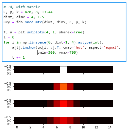
Here are four models of heat transfer, represented numerically, and analytically by the diffusion partial differential equation (PDE). The methods are primarily referenced from Cengel's[1] Heat and Mass Transfer chapters on numerical methods[1]. First are the numerical representations of transient heat conduction, written first with for loops and then rewritten with matrix transformations. 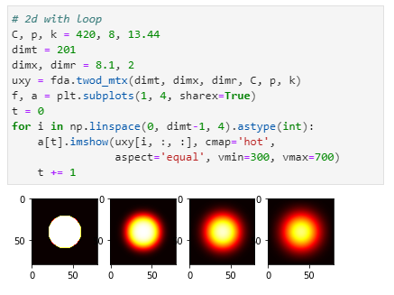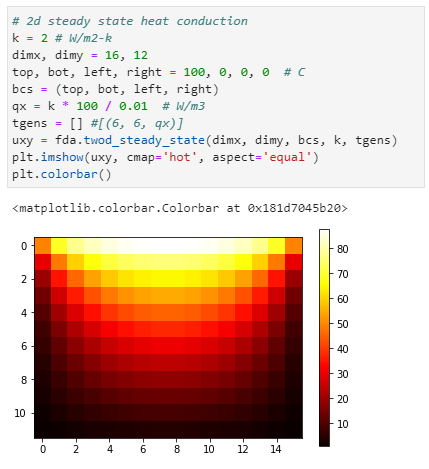First, in 1D, with a heat source in the middle iterated for four timesteps: Then the same model extended to 2D, again with a heat source in the middle iterated for four timesteps: Next, the models of the steady-state equivalent. While I could have recycled my previous numerical methods again, and just iterated the heat transfer until it converges to its steady-state, I decided to use the more efficient analytical solution, since steady-state systems can be analytically solved as a linear system of equations. The trick here was to construct an N x N matrix for N nodes that can model the heat flow into each node from it's four neighbors. Here is an example of a 2 x 4 lattice of nodes: N1 N2 N3 N4 N5 N6 N7 N8 This can be modeled with the following matrix: N1 N2 N3 N4 N5 N6 N7 N8 N1 -4 1 0 0 1 0 0 0 = -Tup - Tleft N2 1 -4 1 0 0 1 0 0 = -Tup N3 0 1 -4 1 0 0 1 0 = -Tup N4 0 0 1 -4 0 0 0 1 = -Tup - Tright ----------------------------------- N5 1 0 0 0 -4 1 0 0 = -Tdown - Tleft N6 0 1 0 0 1 -4 1 0 = -Tdown N7 0 0 1 0 0 1 -4 1 = -Tdown N8 0 0 0 1 0 0 1 -4 = -Tdown - Tright Each row models the energy balance for each node, which, as this is a steady state system, equals zero for each node. For boundary nodes (which are all the nodes in the example above), known boundary conditions are moved to the right hand side. Note that between N4 and N5 the boundary conditions are modified to reflect there is no spatial adjacency between them. Setting this as a coefficient matrix \(A\), and boundary conditions and other known states captured in a N x 1 vector \(y\), solving for \(x\) provides the N temperatures. 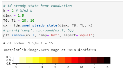\( \begin{align} &A x = y \\ &A^{-1} A x = A^{-1} y \\ &x = A^{-1} y \\ \end{align} \) Here's the 1D versions, with a constant temperature gradient along the x-axis, with only one instance since there's no temporal dimensions to iterate through: Then the same model extended to 2D, with the tempeature gradient aligned to the y-axis: Footnotes 1. Cengel, Yunus A., and Afhsin J. Ghajar. Heat and Mass Transfer: Fundamentals & Applications. New York, 2011. Chapter 5.